


Machining is up to now the most frequently used method of shaping parts of machines and devices in various branches of industry. At present, one can observe a continuous development of this type of machine tools, which is conditioned above all by the growing technological requirements for the manufactured parts.
The dynamic development of this industry is due to the increasing possibilities of computer systems and non-standard construction solutions, which allow the design of multi-purpose machine tools with ever-increasing technological and production resources.
The continuous improvement of Computer Numerically Controlled machine tools and their increasing prevalence has made knowledge of their operation and programming methods a very valuable skill.
To better understand how to program tool movements, it is first necessary to explain the phrase CNC machine programming. This term stands for the creation of a programme which controls the units of a machine tool, which is written in a suitable format and language compatible with the machine’s controller. Format and language need to be compatible with its controller.
For commercially available control types such as Fanuc, Sinumerik, and Heidenhain, the declaration of tool motion works on the same principle as shown in Figure 1 below.
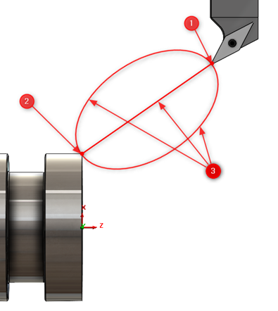
Figure 1. Components of a tool movement description
In order to include a complete description of the movement, it is necessary to specify:
a) The starting point – (1),
b) The end point – (2),
c) Speed,
d) Track – (3).
Programming of tool movements takes place in a continuous manner, and in blocks the final coordinates of movement are given, which means that the end point of movement for a given block of the program is at the same time the starting point of movement for the next block. This principle can be adopted when the machine tool operates in automatic mode executing successive blocks of the program, without intervention of the operator in position of the tool. This principle cannot be applied in semi-automatic mode (e.g. MDI), where the starting point will be the current position of the tool in the working space. Speeds are assigned according to the type of motion programmed.
When using fast movements (G0, F MAX), the speed is taken from the machine data, where the manufacturer has assigned a possible maximum value, and it can usually only be changed from the machine panel using a potentiometer. The speeds of the motions include G1 are declared using the corresponding address F, whose task is to transmit information about the programmed speed to the machine tool controller. As in the case of fast movements, it is also usually possible to correct the speed value on the control panel during the process.
Crucial in determining the motion of a tool is its trajectory, or more precisely the shape of the path the tool takes between certain points. The motion path is referred by the term interpolation, whose task is to independently relate the movements of the required machine axes in order to achieve the resultant motion path of the tool reference point (Figure 2). The machine controller, having known the specified coordinates of the end of the movement and the speed at which it is to take place, is able, using an appropriate module, to calculate the speed vectors of the individual axes.
The drive systems of the required controlled axes receive independent signals so that they work together to move the tool feature point along a defined path to the end point declared in the block.
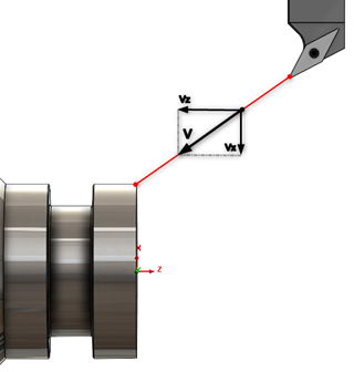
Figure 2: The interpolation vector and its components
Point interpolation – G0
Point interpolation is usually referred to as rapid motion, and in industry this is the term most commonly used. It is based on moving the machine tool units with the fastest possible motion, in such a way that the programmed tool point reaches the final coordinate in the shortest possible time. This type of function is usually used to reach set points that are intended to position the tool accordingly.
The movement to the destination using G0 point interpolation is always along the shortest path (Figure 3) and at full speed, so it is important to program these movements carefully and carefully because a possible collision can have very negative consequences.
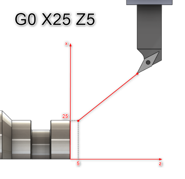
Figure 3. Point interpolation G0
Linear interpolation – G1
G1 linear interpolation is the most commonly used workflow when programming Computer Numerically Controlled (CNC) machine tools. The end point declared in the previous block becomes the start point of the next block.
Starting from these coordinates, the tool travels in a straight line to the declared end coordinates with the programmed feed rate F (Figure 4).
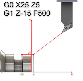
Figure 4. Linear interpolation G1
Interpolacja kołowa – G2/G3
In the case of circular interpolation, knowledge of only two movement points – the beginning and the end does not allow unambiguous definition of movement along the arc of a circle. For that reason it is necessary to define an additional parameter which will make it possible to build an appropriate tool path. In case of circular interpolation this additional parameter is usually the radius of the arc R.
Having known the coordinates of the beginning and the end of the arc, as well as the value of its radius, it is then necessary to decide which type of circular interpolation will be appropriate in a given case. Setting up an appropriate function has an influence on the direction of the created arc and at the same time on the position of the point of its radius.
The distinctions are:
a) G2 – clockwise circular interpolation (CW),
b) G3 – counter-clockwise circular interpolation (CCW).
In the case of milling, it is necessary to determine the correct working plane in order to determine the circular direction (Figure 5).
This selection is made using appropriate preparatory functions such as:
a) G17 – main XY plane,
b) G18 – ZX principal plane,
c) G19 – YZ major plane.
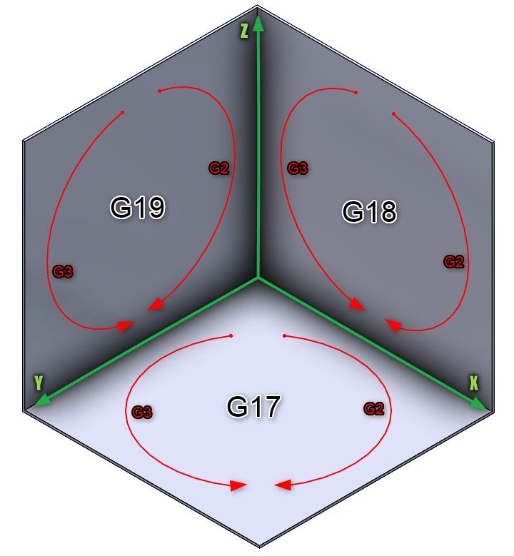
Figure 5: Determination of G2/G3 arc direction for milling on specific working planes
In the case of turning, the direction of circular motion depends primarily on the location of the tool head on the machine tool. When using a tool from the top tool holder which is “above axis” of the workpiece, the directions of motion along the arc of the circle are defined as in figure 6a. The opposite case, which uses a tool from the front head (“under-axis” turning) is described in Figure 6b.
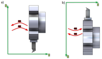
Figure 6 Determination of the G2/G3 arc direction for turning: a) tool position over the Z axis, b) tool position under the Z axis
As in the case of circular interpolation programming it is required to define the radius of the created arc, its description can be done in several ways. The most common methods of defining the radius are:
a) Defining the centre of the circle
This is one of the ways that fully enables the definition of an arc-shaped toolpath. The interpolation parameters I, J, K, with which the centre of the circle is programmed, are defined for the relevant axes in the given active machining plane.
The I parameter is responsible for the X axis, the J for the Y axis and the last K analogously for the Z axis.
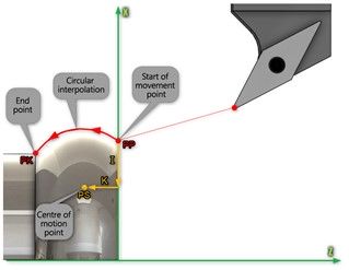
Figure 7 Parameters I and K defining the centre of the arc
The method described above for defining circular interpolation with indicating the centre of the circle by parameters I, J, K is often used and recommended method of creating circular interpolation. By specifying these values the user avoids the need to recalculate and determine the coordinates of the centre of the circle by the control system as it happens with other methods.
b) Direct programming of the circle radius
For industrial detail documentation where there are surfaces that need to be programmed using circular interpolation, these are usually described using radial or diameter dimensions. Circular interpolation programming using radius definition (Figure 8) is therefore a faster and more user-friendly method. Based on the radius declared in the control code, the control system itself determines the position of the circle centre.
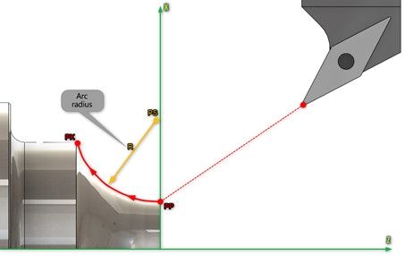
Figure 8. Defining circular interpolation using radius
In addition, the radius value can be given with a positive or negative sign, which determines the selection of the tool path along a shorter or longer arc of the circle. The sign depends on the size of the angle for which the arc is spread. Referring to Figure 9, for a positive value of the radius, the tool will run on an angle smaller or equal to 180°. For a negative value, the tool will move through an angle greater than 180°.
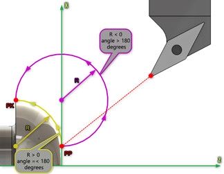
Figure 9 Determination of the G2/G3 arc direction for turning: a) tool position over the Z axis, b) tool position under the Z axis
In addition to the above-mentioned and most commonly used ways of declaring a radius, there are additional ways whose presence and manner of definition depends on the type of control.
Some examples include:
a) Programming with definition of the angle of the arc,
b) Programming of the angle and centre of the arc,
c) Programming by intermediate point
d) Programming with definition of the tangent arc,
e) Programming of full circle arc.
Tool radius correction
An important factor to mention when programming tool paths is their correction, which is sometimes also called compensation. How much more difficult it would be to program workpiece contours where the user would have to take a correction for the tool being used and offset the programmed contour by the value of its radius.
Bearing in mind that tools are not solid blocks with ideal shapes and dimensions, which can often change as a result of e.g. wear, how much work would it be to change the contour by a hundredth of a millimetre to achieve the desired dimensional tolerances? Fortunately, there are suitable preparation functions (G41 and G42) that automatically read off the necessary information from the tool table.
Figure 10 shows an example of tool radius correction on a turning machining example. Due to the roundness of the tool insert, the motion path had to be offset by the radius value in order to produce the programmed contour in the correct dimensions.
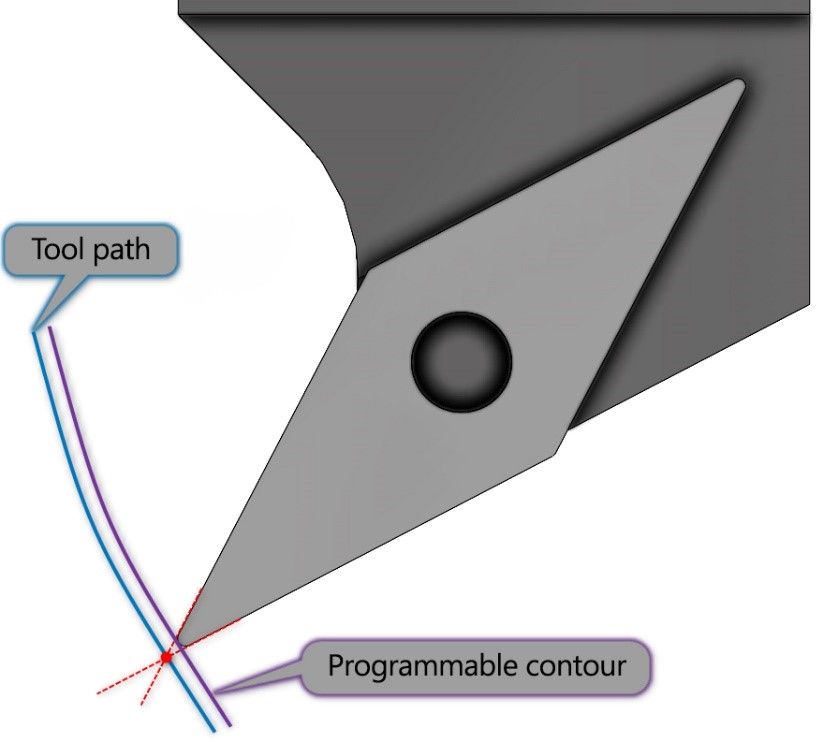
Figure 10 Tool radius compensation using lathe machining as an example
Currently there are two methods of programming tool radius correction:
a) Programme
Industry now makes large use of CAM systems that allow the creation of machining programmes together with simulation of the full process of making parts on CNC machines. This software also has a radius correction module, which enables the generation of a G-code with coordinates altered by the radius value of the tool being used.
The advantage of this solution is that the full verification of the generated control code can take place before it is run on the machine, but any changes due to tool condition require the modified program to be generated again. This solution is ideal for machining free surfaces where it is necessary to use spatial compensation.
b) Automatic
The correction is made by the machine tool controller, which reads the relevant data about the tool in use from the tool table. This has a great impact on machining accuracy, as even the smallest changes in tool dimensions can be entered in real time by the operator and taken into account by the machine tool controller at each subsequent programme run.
To generate an appropriate motion path considering the tool geometry, the preparatory functions G specified for this purpose are used (Figure 11): G40 – disable automatic tool radius correction (motion path following the contour), G41 – enable automatic tool radius correction to the left of the programmed contour (tool position to the left of the programmed contour looking in the direction of motion), G42 – enable automatic tool radius correction to the right of the programmed contour (tool position to the right of the programmed contour looking in the direction of motion).
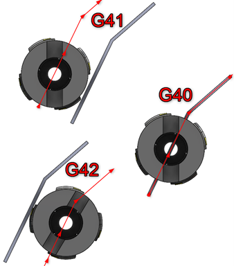
Figure 11 Programming of automatic tool radius correction
Defining the tool path is a basic element of each program, without which we would not be able to make any workpiece on CNC machine tools.
The use of G0 point interpolation, by means of which, for example, the tool positioning movements required for their correct positioning are defined, provides great time savings due to working at maximum speeds. G1 linear interpolation and G2/G3 circular interpolation are functions that create working movements of a tool for machining workpieces of various purposes. They are the basis of programs for machines of various types and designs, from simple lathes and milling machines to lathes with a sub-spindle and several tool heads, up to five-axis milling centres making the most complex surfaces. The principle behind them is that all the machining cycles available in the machine tool controllers of various manufacturers are based on dialogue programming.
Tool correction is also an important programming aspect that makes it easy to adjust the tool path in relation to its geometry, and the possibility of correcting values and taking into account tool wear makes it possible to produce parts where shape-dimensional accuracy is of paramount importance.


![By 2030, the market size of metal processing tools is expected to reach $120.44 billion [REPORT]](https://industryinsider.eu/wp-content/uploads/xcutting-tools-320x167.jpg.pagespeed.ic.SgnEk-RWA-.jpg "By 2030, the market size of metal processing tools is expected to reach $120.44 billion [REPORT]")